Advanced R for Econometricians

Advanced R for EconometriciansFunctional Style R ProgrammingMartin C. Arnold, Jens Klenke1 / 40

Part I

Functional Programming Using purrr

2 / 40

Functional Style Programming
To become significantly more reliable, code must become more transparent. In particular, nested conditions and loops must be viewed with great suspicion. Complicated control flows confuse programmers. Messy code often hides bugs.
— Bjarne Stroustrup
3 / 40

FAQs

# Packages needed
library(dplyr)
library(purrr)
library(readr)
# (or simply attach the tidyverse!)

What is a functional programming (FP) language?

Simply put: a language which is centered on problem-solving using functions!
There are two common threads in FP:
1. A functional language has first-class functions which behave like any other data type. In R this means we may treat function like variables (i.e., assign them, store them in a list or pass them as arguments to other functions)
2. Many functional languages require pure functions only. These are functions which have no side-effects: they do not interfere with anything outside their scope and produce output which depends only on the input.

4 / 40

R has first-class functions.
Does R allow for pure functions only? No: e.g. print() has side-effects. Obviously all functions which return pseudo-random numbers are not pure functions.

FAQs

Is R a FP language?

R is not a FP language but we may adopt a functional style of programming.
Functionals are functions which take functions as input and produce, e.g. vector output

Why should I use functional style programming?

FP is often space efficient, very comprehensible and easily adopted to new situations
Functionals are easily analysed in isolation and thus are often straightforward to optimise and parallelise

(We'll discuss functionals in a minute)

5 / 40

You've probably used functionals already: lapply() and integrate() are prominent examples.

FAQs

What does 'FP style' even mean?

It’s hard to describe exactly what a functional style is, but generally we will refer to the following definition:

Functional programming style means decomposing a big problem into smaller pieces, then solving each piece with a function or combination of functions. — Hadley Wickham

6 / 40

FAQs

We will briefly discuss key techniques in functional R programming which are best summarised by the table below. We will focus on purrr functionals and applications of function factories.

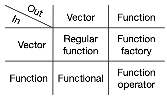
Source: Wickham (2019)

7 / 40

Functionals

A functional takes a function as an input and returns a vector as output.

Let's do something that might seem strange at first sight:

randomise <- function(f) f(rnorm(1e3))
randomise(mean)

## [1] -0.002711432

randomise(sum)

## [1] -75.23842

8 / 40

Functionals can also produce other data structures, e.g., data frames as output.

Functionals

Functionals are often used as alternatives to loops. Not because loops are inherently slow (which is common wisdom), but because loops
- make it relatively cumbersome to harness the power of iteration
- are prone to typos that are difficult to identify
- can be overly flexible: loops convey that an iteration is done, but may make it relatively hard to grasp what is done and what should be done with the results.
Functionals are tailored to specific tasks which immediately convey why they are being used and what output format they produce.
Switching from loops to functionals doesn't necessarily mean that we must write our own functionals: the purrr package provides functionals which are very easy to apply and also fast as they are written in C.

9 / 40

With functionals we don't need to worry about indexing, brackets, curly braces etc.
Of course, flexibility isn't bad. They idea of a FP is to use functionals that perform a specific iteration which returns a specific output format.
Others are likely to be puzzled by looking at your code if it uses a lot of loops. Functionals immediately convey which iteration is done and which output is returned.

'Others' also includes your future self :-)

Functionals — `purrr::map()`

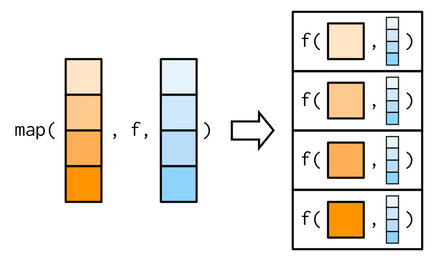
map() is the purrr version of lapply().

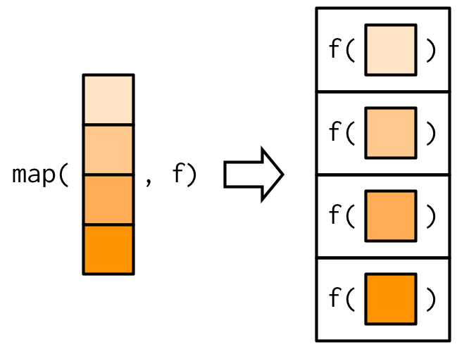
Source: Wickham (2019)

Example: `map()`

map(1:3, f) is list(f(1), f(2), f(3)).

triple <- function(x) x * 3
map(1:3, triple)

## [[1]]
## [1] 3
## 
## [[2]]
## [1] 6
## 
## [[3]]
## [1] 9

10 / 40

Do the example using lapply(): lapply(1:3, function(x) x * 3)
Obviously map() returns a list, too.

`purrr::map_*()` — Producing Atomic Vectors

There are helper functions which are more convenient if simpler data structures are required: map_lgl(), map_int(), map_dbl(), and map_chr() return an atomic vector of the specified type
Base R equivalents are sapply() and vapply()

Example: `map_*()`

Source: Wickham (2019)

# check class of mtcars data
class(mtcars)

## [1] "data.frame"

map_lgl(mtcars, is.double)

##  mpg  cyl disp   hp drat   wt qsec   vs   am gear carb 
## TRUE TRUE TRUE TRUE TRUE TRUE TRUE TRUE TRUE TRUE TRUE

n_unique <- function(x) length(unique(x))
map_int(mtcars, n_unique)

##  mpg  cyl disp   hp drat   wt qsec   vs   am gear carb 
##   25    3   27   22   22   29   30    2    2    3    6

11 / 40

Remember that logical, integer, double and character are atomic types
mtcars is a data frame thus the map_*() functions map the columns
Of course, the * in map_*() must match the return type of the functions used for mapping

`purrr::map_*()` — Producing Atomic Vectors

The twiddle operator ~ allows to write anonymous functions in a less verbose manner. It conveys that the subsequent expression is a formula.
A good rule of thumb: if a function spans lines or uses {...}, we should give it a name.

Example: `map_*()` with inline anonymous function

map_dbl(mtcars, function(x) length(unique(x)))

##  mpg  cyl disp   hp drat   wt qsec   vs   am gear carb 
##   25    3   27   22   22   29   30    2    2    3    6

map_dbl(mtcars, ~ length(unique(.x)))

##  mpg  cyl disp   hp drat   wt qsec   vs   am gear carb 
##   25    3   27   22   22   29   30    2    2    3    6

12 / 40

`purrr::map_*()` — Producing Atomic Vectors

map_*() is useful for selecting elements from a list by name, position, or both.

Example: element extraction with `map_*()`

x <- list(
  list(-1, x = 1, y = c(2), z = "a"),
  list(-2, x = 4, y = c(5, 6), z = "b"),
  list(-3, x = 8, y = c(9, 10, 11))
)

map_dbl(x, "x")   # select by name

## [1] 1 4 8

map_dbl(x, 1)     # select by position

## [1] -1 -2 -3

13 / 40

In base R we'd have to write a function that iterates through x or use sapply().

`purrr::map_*()` — Producing Atomic Vectors

Task:

Write short Base R code which works on x from the previous slide and returns

all entries named 'x' and
all entries at position 1 from this nested list.

14 / 40

# 1.
sapply(x, "[[", "x")
# 2.
sapply(x, "[[", 1)

## [1] 1 4 8
## [1] -1 -2 -3

`purrr::map_*()` — Producing Atomic Vectors

Note that components must exist in all entries of the object we iterate over (here a nested list).

Example: element extraction with `map_*()`

map_chr(x, "z")   # z doesn't exist in x[[3]]

## Error in `stop_bad_type()`:
## ! Result 3 must be a single string, not NULL of length 0

To prevent this error a .default value can be supplied.

map_chr(x, "z", .default = NA)

## [1] "a" "b" NA

15 / 40

Keep in mind that this requires your subsequent code to work with NAs.

`purrr::map_*()` — Producing Atomic Vectors

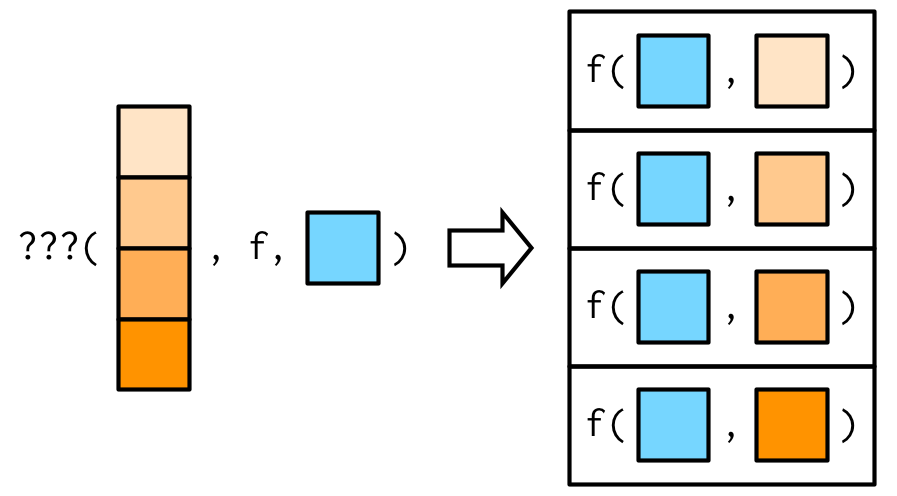
Additional arguments to the mapping function may be passed after the function name.
We need to be careful with evaluation!

Example: mapping with additional arguments

Source: Wickham (2019)

x <- list(1:5, c(1:10, NA))
map_dbl(x, ~ mean(.x, na.rm = TRUE))

## [1] 3.0 5.5

More efficient:

map_dbl(x, mean, na.rm = TRUE)

## [1] 3.0 5.5

16 / 40

Arguments passed to an anonymous function are evaluated in every iteration. The latter approach is more efficient because additional arguments are evaluated just once.

`purrr::map_*()` — Producing Atomic Vectors

Additional arguments are not decomposed: map_*() is only vectorised over (the data passed as) the first argument. Further (vector) arguments are passed along.

Example: mapping with additional arguments — ctd.

Source: Wickham (2019)

# Arg. 'mean' is recycled
map(1:3, rnorm, mean = c(100, 10, 1))

## [[1]]
## [1] 101.1215
## 
## [[2]]
## [1] 101.324174   9.246503
## 
## [[3]]
## [1] 101.8168982  10.5856532   0.9970042

17 / 40

Question to students:

Explain the outcomes of map(1:4, rnorm, mean = c(100, 10, 1))

`purrr::map_*()` — Producing Atomic Vectors

Example: mapping over a different argument

Assume you'd like to investigate the impact of different amounts of trimming when computing the mean of observations sampled from a heavy-tailed distribution.

Source: Wickham (2019)

trims <- c(0, 0.1, 0.2, 0.5)
x <- rcauchy(1000)

We may switch arguments using an anonymous function:

map_dbl(trims, ~ mean(x, trim = .x))

## [1] 0.624460050 0.006129521 0.038663335 0.075093275

This is equivalent to:

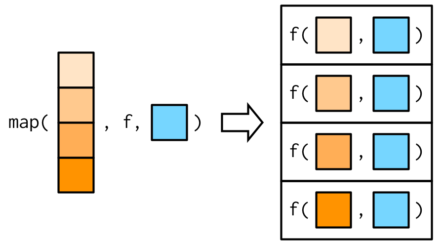
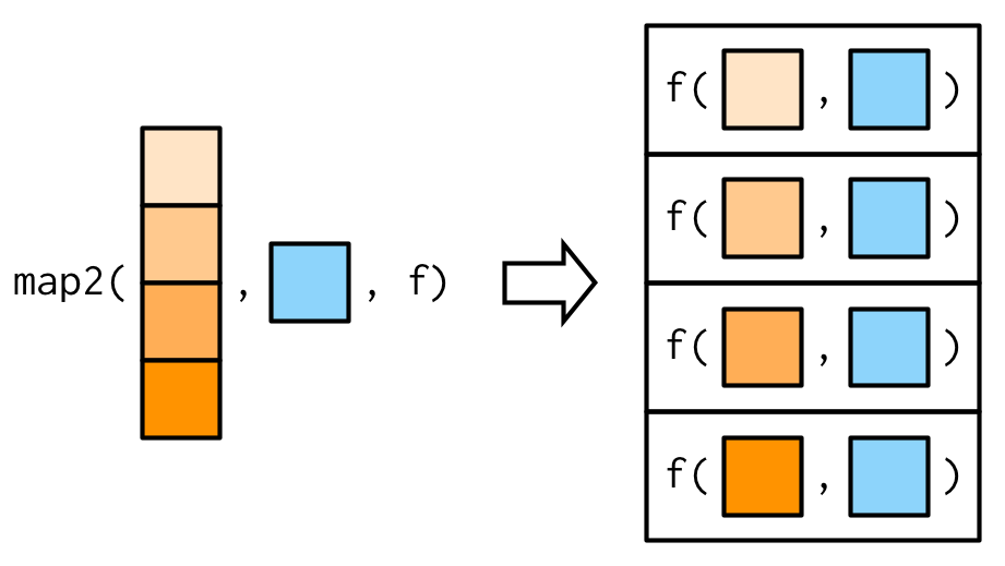
map_dbl(trims, function(trim) mean(x, trim = trim))

## [1] 0.624460050 0.006129521 0.038663335 0.075093275

18 / 40

`purrr::map_*()` — Exercises

map(1:3, ~ runif(2)) is a useful pattern for generating random numbers, but map(1:3, runif(2)) is not. Why not? Can you explain why it returns the result that it does?
The following code simulates the performance of a t-test for non-normal data. Extract the p-value from each test, then visualise.
```
trials <- map(1:100, ~ t.test(rpois(10, 10), rpois(10, 7)))
```
Use map() to fit linear models to the mtcars dataset using the formulas stored in this list:
```
formulas <- list(
   mpg ~ disp,
   mpg ~ disp + wt,
   mpg ~ I(1 / disp) + wt
)
```

19 / 40

map(1:3, ~ runif(2)) evaluates runif() with n = 2 in every iteration since ~ converts to an anonymous function. map(1:3, runif(2)) evaluates runif(2) only once and cannot do mapping because runif(2) is not treated as a function. NULL is returned in every iteration.

Code:

library(ggplot2)
trials_df <- tibble(p_value = map_dbl(trials, "p.value"))
trials_df %>% 
  ggplot(aes(x = p_value, fill = p_value < 0.05)) + 
  geom_histogram(binwidth = .025) +
  ggtitle("Distribution of p-values for random Poisson data.")

Code:

models <- map(formulas, lm, data = mtcars)

Case Study: Model Fitting with `purrr`

Tired of mtcars? We're too... let's use cars2018, a dataset on fuel efficiency of real cars of today from a US Department of Energy instead! 🚗🚗🚗

We will now take a look at how purrr functions can be used to fit a regression model to subgroups of data, extract estimates and then compare the approach to base R approaches.

Instructions

Load the cars2018.csv dataset and split it by Drive, see ?split
Use purrr (preferably together with dplyr) to
- fit the model MPG ~ Cylinders to each subgroup
- extract the estimated coefficient of Cylinders
Contrast your purrr approach to base R alternatives that rely on *apply() and for(), respectively

20 / 40

Map Variants

There are 23 variants of map*() which are easily understood as variants of the following functions:

Output same type as input: modify()
Iterate over two inputs: map2()
Iterate with an index: imap()
Return nothing: walk()
Iterate over any number of inputs: pmap()

	List	Atomic	Same type	Nothing
One argument	`map()`	`map_*()`	`modify()`	`walk()`
Two arguments	`map2()`	`map2_*()`	`modify2()`	`walk2()`
One argument + index	`imap()`	`imap_*()`	`imodify()`	`iwalk()`
N arguments	`pmap()`	`pmap_*()`	`—`	`pwalk()`

21 / 40

The table shows input (rows) and output types (columns).

`purrr::modify()`

The modify() function works on the input components and returns an object of the same type as the input.

Example: `data.frame` in / `data.frame` out

df <- data.frame(
  x = 1:3,
  y = 6:4
)
modify(df, ~ .x * 2)

##   x  y
## 1 2 12
## 2 4 10
## 3 6  8

Note that modify() never modifies in-place but creates a copy, which must be (re)assigned.

df <- modify(df, ~ .x * 2)

22 / 40

`purrr::map2()`

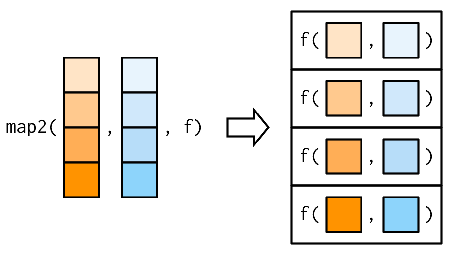
map2() is vectorised over two arguments.

Example: weighted mean using `map2()`

Source: Wickham (2019)

Let's generate lists of observations and associated weights.

set.seed(123)
xs <- map(1:4, ~ runif(4))
xs[[1]][[1]] <- NA
ws <- map(1:4, ~ rpois(4, 5) + 1)

map2_dbl varies both xs and ws as inputs to weighted.mean().

map2_dbl(xs, ws, weighted.mean)

## [1]        NA 0.6625391 0.5968213 0.5287878

23 / 40

`purrr::map2()`

Additional arguments may be passed just as with map().

Example: weighted mean using `map2()` — ctd.

Source: Wickham (2019)

# passing na.rm = TRUE
map2_dbl(xs, ws, weighted.mean, na.rm = TRUE)

## [1] 0.7355541 0.6625391 0.5968213 0.5287878

24 / 40

`purrr::map2()`

Note that map2() also recycles inputs to ensure that they are the same length.

Example: weighted mean using `map2()` — ctd.

Source: Wickham (2019)

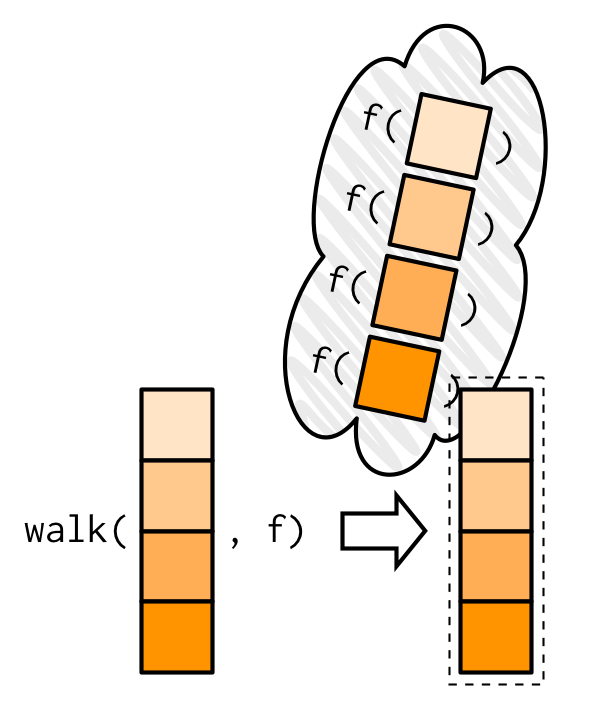
map2_dbl(1:6, 1, ~ .x + .y)

## [1] 2 3 4 5 6 7

25 / 40

`purrr::walk()`

walk() ignores the return value of .f and returns .x invisibly. This is useful for functions that are called for their side-effects.
There is no base R equivalent but wrapping lapply() with invisible() comes close

Example: assigning and passing objects

Source: Wickham (2019)

Assignment to an environment is a side-effect.

26 / 40

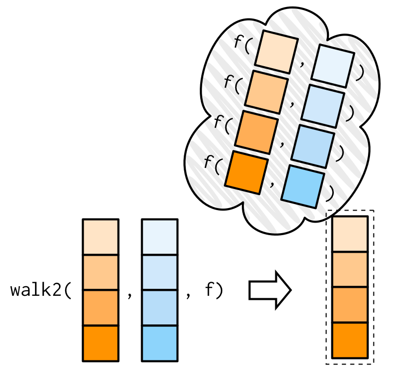
`purrr::walk()`

walk2() is a convenient alternative which is vectorised over two arguments.

Example: write to disc

Source: Wickham (2019)

A common side-effect which needs two arguments (object and path) is writing to disk.

27 / 40

`purrr::imap()`

map(.x, .f) is essentially an analog to for(x in xs) <apply .f to x and assign to list>
for(i in seq_along(xs)) and for(nm in names(xs)) are analogous to imap():

imap(.x, .f) applies .f to values .x and indices or names derived from .x.

Example: named column means

imap() is a useful helper if we want to work with values along with variable names.

28 / 40

When using the formula shortcut, the first argument .x is the value, and the second .y is the position/name
cars2018 %>% select_if(is.numeric) returns a list so .y is a name and .x the value
character vectors index by name, numeric vectors index by position

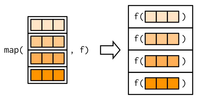
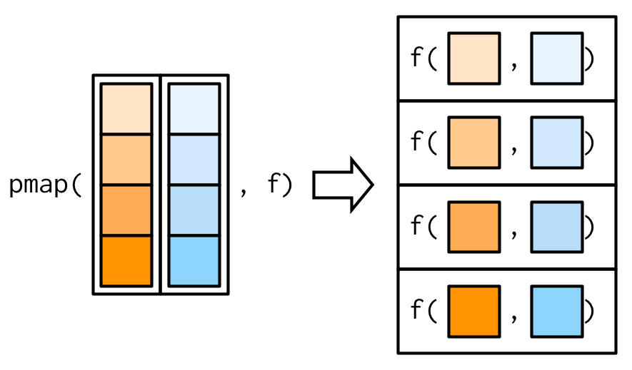
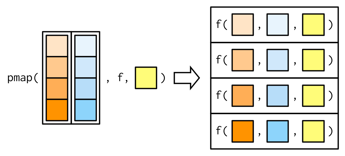
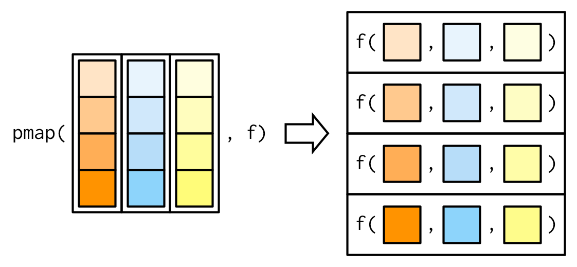
`purrr::pmap()`

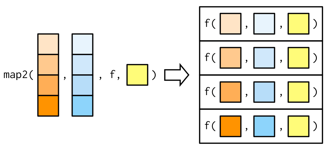
pmap() generalises map() and map2() to p vectorised arguments. Thus pmap(list(x, y), f) is the same as map2(x, y, f).

Example: weighted mean with `pmap()`

Source: Wickham (2019)

map2_dbl() behaves as pmap_dbl() in the two-argument case:

map2_dbl(xs, ws, weighted.mean)

## [1]        NA 0.6625391 0.5968213 0.5287878

pmap_dbl(list(xs, ws), weighted.mean)

## [1]        NA 0.6625391 0.5968213 0.5287878

29 / 40

`purrr::pmap()`

As before, additional arguments may be passed after .f and they are recycled, if necessary.

Example: weighted mean with `pmap()` — ctd.

Source: Wickham (2019)

Now with the additional argument na.rm = TRUE:

pmap_dbl(list(xs, ws), 
         weighted.mean, 
         na.rm = TRUE)

## [1] 0.7355541 0.6625391 0.5968213 0.5287878

30 / 40

`purrr::pmap()`

Note that pmap() gives much finer control over argument matching as we may use named list. This is very convenient for working with complex list objects.

Example: argument matching using named list

Source: Wickham (2019)

We look at the trimmed mean example again.

trims <- c(0, 0.1, 0.2, 0.5)
x <- rcauchy(1000)

Varying the trim argument can be done by passing the values in a named list.

pmap_dbl(list(trim = trims), mean, x = x)

## [1] -0.03231537  0.06072652  0.04464511  0.04482772

31 / 40

`purrr::pmap()`

Remember that a data.frame is a list and thus can be passed to pmap() as a collection of inputs.

Example: `pmap()` with data.frame as input

Source: Wickham (2019)

params <- tibble::tribble(
  ~ n, ~ min, ~ max,
   1L,     0,     1,
   2L,    10,   100
)

Column names match the arguments: we don't have to worry about their order.

pmap(params, runif)

## [[1]]
## [1] 0.4475701
## 
## [[2]]
## [1] 21.72593 65.95534

32 / 40

tribble(): create tibbles using an easier to read row-by-row layout. This is useful for small tables of data where readability is important.

`purrr::pmap()` — Exercises

Explain the results of modify(cars2018, 1)

Explain how the following code transforms a data.frame using functions stored in a list.

trans <- list(
  Displacement = function(x) x * 0.0163871,
  Transmission = function(x) factor(x, labels = c("Automatic", "Manual", "CVT"))
)
nm <- names(trans)
cars2018[nm] <- map2(trans, cars2018[nm], function(f, var) f(var))

Compare and contrast the map2() approach to this map() approach:
```
cars2018[nm] <- map(nm, ~ trans[[.x]](cars2018[[.x]]))
```

33 / 40

modify() is a shortcut for x[[i]] <- f(x[[i]]); return(x). So every row is filled with it's first value.
Too lenghty, see class notes
As above

Part II

Function Factories

34 / 40

Function Factories

A function factory is a function that produces functions.

Example: function factory

nth_root <- function(n) {   # function factory
  function(x) {
    x^(1/n)
  }
}
cube_root <- nth_root(3)    # manufactured function
cube_root(8)

## [1] 2

35 / 40

Function Factories

The enclosing environment of the manufactured function is an execution environment of the function factory.

Example: function factory — ctd.

rlang::env_print(cube_root)     # inspect enclosing environment

## <environment: 0x1043a9fa8>
## Parent: <environment: global>
## Bindings:
## • n: <dbl>

rlang::fn_env(cube_root)$n      # retrieve from enclosing environment

## [1] 3

36 / 40

Remember that execution environments are ephemeral in general: they are destroyed once the function has run.
This is different here: the enclosing environment of cube_root() was the execution environment of nth_root()—a mechanism which makes function factories possible.

Function Factories

Remember lazy evaluation?

Example: function factory — ctd.

n <- 2
sq <- nth_root(n)
n <- 16
sq(64)             # Wait... this should evaluate to 8!

## [1] 1.29684

37 / 40

64^(1/16) = 1.29684
x is lazily evaluated when sq() is run, not when nth_root() is run. We thus need to force evaluation.
This is likely to happen so it's a good practice to avoid such a bug by using force() in your factories!

Function Factories

Remember lazy evaluation?

Example: function factory — ctd.

nth_root <- function(n) {
    force(n)
    function(x) {
      x^(1/n)
    }
}
n <- 2
sq <- nth_root(n)
n <- 16
sq(64)             # better :-)

## [1] 8

38 / 40

Question to students: why force(x) and not just x? (check def. of force()
Note on Garbage Collection:

As manufactured functions hold on to the execution environment of the function factory you need to remove large objects manually.
```
f1 <- function(n) {
x <- runif(n)
m <- mean(x)
rm(x) # use lobstr::obj_size() on a man. function to see difference
function() m
}
```

Function Factories — Stateful Functions

Function factories allow us to create functions with a memory.

Example: counter

# factory for a counter
new_counter <- function() {
  i <- 0
  function() {
    i <<- i + 1
    i
  }
}
counter_one <- new_counter()
counter_two <- new_counter()
replicate(2, counter_one())

## [1] 1 2

replicate(5, counter_two())

## [1] 1 2 3 4 5

39 / 40

Should be used with moderation. The S6 system is more suitable if your manufactured functions are to manage multiple variables.
The "state" (i here) is tracked in the execution environment. This is a different environment for each function produced by the factory.
```
rlang::env_print(counter_one)
rlang::env_print(counter_two)
```

Thank You!

40 / 40

Help

Keyboard shortcuts

↑, ←, Pg Up, k

Go to previous slide

↓, →, Pg Dn, Space, j

Go to next slide

Home

Go to first slide

End

Go to last slide

Number + Return

Go to specific slide

b / m / f

Toggle blackout / mirrored / fullscreen mode

Clone slideshow

Toggle presenter mode

Restart the presentation timer

?, h

Toggle this help

Advanced R for Econometricians

Functional Style R Programming

Martin C. Arnold, Jens Klenke

Part I

Functional Style Programming

FAQs

FAQs

FAQs

FAQs

Functionals

Functionals

Functionals — purrr::map()

Example: map()

purrr::map_*() — Producing Atomic Vectors

Example: map_*()

purrr::map_*() — Producing Atomic Vectors

Example: map_*() with inline anonymous function

purrr::map_*() — Producing Atomic Vectors

Example: element extraction with map_*()

purrr::map_*() — Producing Atomic Vectors

purrr::map_*() — Producing Atomic Vectors

Example: element extraction with map_*()

purrr::map_*() — Producing Atomic Vectors

Example: mapping with additional arguments

purrr::map_*() — Producing Atomic Vectors

Example: mapping with additional arguments — ctd.

purrr::map_*() — Producing Atomic Vectors

Example: mapping over a different argument

purrr::map_*() — Exercises

Case Study: Model Fitting with purrr

Map Variants

purrr::modify()

Example: data.frame in / data.frame out

purrr::map2()

Example: weighted mean using map2()

purrr::map2()

Example: weighted mean using map2() — ctd.

purrr::map2()

Example: weighted mean using map2() — ctd.

purrr::walk()

Example: assigning and passing objects

purrr::walk()

Example: write to disc

purrr::imap()

Example: named column means

purrr::pmap()

Example: weighted mean with pmap()

purrr::pmap()

Example: weighted mean with pmap() — ctd.

purrr::pmap()

Example: argument matching using named list

purrr::pmap()

Example: pmap() with data.frame as input

purrr::pmap() — Exercises

Part II

Function Factories

Example: function factory

Function Factories

Example: function factory — ctd.

Function Factories

Example: function factory — ctd.

Function Factories

Example: function factory — ctd.

Function Factories — Stateful Functions

Example: counter

Thank You!

Part I

Help

Functionals — `purrr::map()`

Example: `map()`

`purrr::map_*()` — Producing Atomic Vectors

Example: `map_*()`

`purrr::map_*()` — Producing Atomic Vectors

Example: `map_*()` with inline anonymous function

`purrr::map_*()` — Producing Atomic Vectors

Example: element extraction with `map_*()`

`purrr::map_*()` — Producing Atomic Vectors

`purrr::map_*()` — Producing Atomic Vectors

Example: element extraction with `map_*()`

`purrr::map_*()` — Producing Atomic Vectors

`purrr::map_*()` — Producing Atomic Vectors

`purrr::map_*()` — Producing Atomic Vectors

`purrr::map_*()` — Exercises

Case Study: Model Fitting with `purrr`

`purrr::modify()`

Example: `data.frame` in / `data.frame` out

`purrr::map2()`

Example: weighted mean using `map2()`

`purrr::map2()`

Example: weighted mean using `map2()` — ctd.

`purrr::map2()`

Example: weighted mean using `map2()` — ctd.

`purrr::walk()`

`purrr::walk()`

`purrr::imap()`

`purrr::pmap()`

Example: weighted mean with `pmap()`

`purrr::pmap()`

Example: weighted mean with `pmap()` — ctd.

`purrr::pmap()`

`purrr::pmap()`

Example: `pmap()` with data.frame as input

`purrr::pmap()` — Exercises