Advanced R for Econometricians
Measuring Performance and Profiling
Martin C. Arnold, Jens Klenke
What's up next? — Overview
Now:
Measuring Performance: Profiling and Microbenchmarking
(Why) is
Rslow?
Remaining classes:
Improving Performance
How to speed things up using
Rcpp(and hopefullyRcppArmadillo)
Profiling
Prerequisites
# packages neededlibrary(profvis)library(bench)library(beeswarm) # for plotting with `bench` packageProfiling means measuring run time of our code line-by-line using realistic inputs in order to identify bottlenecks.
After identifying bottlenecks we experiment with alternatives and find the fastest using a microbenchmark.
We will use the packages
profvisandbenchfor profiling and benchmarking.
It’s tempting to think you just know where the bottlenecks in your code are. I mean, after all, you write it! But trust me, I can’t tell you how many times I’ve been surprised at where exactly my code is spending all its time. The reality is that profiling is better than guessing. — Roger D. Peng
Profiling — utils::Rprof()
Rprof()is a build-in sampling profiler. It keeps track of the function call stack at regularly sampled intervals.Note: results are stochastic—we never run a function under the same conditions twice (think memory usage, CPU load, etc.)
Example: profiling a call of replicate()
tmp <- tempfile()Rprof(tmp, interval = 0.1) # start the profilerreplicate(5, mean(rnorm(1e6)))Rprof(NULL) # stop profilingwriteLines(readLines(tmp))## ## sample.interval=100000## "rnorm" "mean" "FUN" "lapply" "sapply" "replicate" ## "rnorm" "mean" "FUN" "lapply" "sapply" "replicate" ## "rnorm" "mean" "FUN" "lapply" "sapply" "replicate"Visualising profiles: profvis::profvis()
Exercise: profiling nested functions
Profile a call of f() and visualise the results using profvis::profvis().
# define some (nested) example functionsf <- function() { pause(0.1) g() h()}g <- function() { pause(0.1) h()}h <- function() { pause(0.1)}Visualising profiles: profvis::profvis()
Example: profiling linear regression
profvis({ dat <- data.frame( x = rnorm(5e4), y = rnorm(5e4) ) plot(x ~ y, data = dat) m <- lm(x ~ y, data = dat) abline(m, col = "red")})Visualising profiles: profvis::profvis()
Example: profiling linear regression
Visualising profiles: profvis::profvis()
Example: profiling linear regression
Memory Profiling
Exercise: extensive garbage collection
The following code generates a large number of short-lived objects by copy-on-modification.
What does profvis() reveal?
profvis({ x <- integer() for (i in 1:1e4) { x <- c(x, i) }})Memory Profiling
Sometimes code statements seem fairly innocent but are very inefficient both when it comes to memory and speed.
Exercise: coercion to another type
Can you explain why execution of the third line needs 762.9MB memory?
profvis({ x <- matrix(nrow = 1e4, ncol = 1e4) x[1, 1] <- 0 x[1:3, 1:3] })Memory Profiling
Exercise: coercion to another type
Profiling — some notes and hints
C/C++(or other compiled) code cannot be profiledWe also cannot profile what happens inside primitive functions, e.g.,
sum()andsqrt()(these functions are written inCorFORTRAN).We thus cannot use profiling to see whether the code is slow because something further down the call stack is slow.
Profiling is another good reason to break your code into functions so that the profiler can give useful information about where time is being spent
Microbenchmarking
What is a Microbenchmark?
"A microbenchmark is a program designed to test a very small snippets of code for a specific task. Microbenchmarks are always artificial and they are not intended to represent normal use."
We usually speak of milliseconds (ms), microseconds (µs), or nanoseconds (ns) here.
Important:
microbenchmarks can rarely be generalised to 'real' code: the observed differences in microbenchmarks will typically be dominated by higher-order effects in real code.
Think of it this way:
A deep understanding of quantum physics is not very helpful when baking cookies.
There are several R packages for microbenchmarking. We will rely on the
benchpackage by Hester (2022) which has the most accurate timer function currently available inR.
Microbenchmarking — the bench package
benchis part of thetidyerse. It uses the highest precision APIs available for the common operating system (often nanoseconds-level!)mark()is the working horse of thebenchpackage and measures both memory allocation and computation time.By default, a human-readable statistical summary on the distributions of memory load and timings based on 1e4 iterations is returned which also reports on garbage collections
Benchmarking across a grid of input values with
bench::press()is possibleThe package also has methods for neat visualisation of the results using
ggplot2::autoplot()(default plot type is beeswarm)
Microbenchmarking — bench::mark()
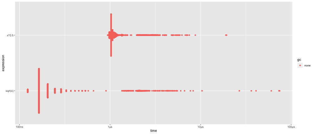
Example: "the fastest square root"
x <- runif(100)(lb <- bench::mark( sqrt(x), x^0.5))## # A tibble: 2 × 6## expression min median `itr/sec` mem_alloc `gc/sec`## <bch:expr> <bch:tm> <bch:tm> <dbl> <bch:byt> <dbl>## 1 sqrt(x) 123ns 164.15ns 3232274. 848B 0## 2 x^0.5 943ns 1.02µs 864867. 848B 0plot(lb)Microbenchmarking — bench::mark()
Example: "the fastest square root"
Microbenchmarking — bench::mark()
Example: non-equivalent code
set.seed(42)dat <- data.frame( x = runif(10000, 1, 1000), y = runif(10000, 1, 1000) )bench::mark( dat[dat$x > 500, ], dat[which(dat$x > 499), ], subset(dat, x > 500) )## ## Error: Each result must equal the first result:## `dat$x > 500` does not equal `which(dat$x > 499)` Each result must ## equal the first result:## `` does not equal ``##Use check = FALSE to disable checking of consistent results.
Microbenchmarking — bench::press()
Sometimes it is useful to benchmark against a parameter grid. This can be done using bench::press().
Exercise: benchmark against parameter grid
Benchmark subsetting functions for dataframes generated by create_df() for combination of rows = c(10000, 100000) and cols = c(10, 100).
create_df <- function(rows, cols) { as.data.frame( matrix( unlist(replicate(cols, runif(rows, 1, 1000), simplify = FALSE)), nrow = rows, ncol = cols ) )}Microbenchmarking — Exercises
Instead of using
bench::mark(), you could use the built-in functionsystem.time()which is, however, much less precise, so you’ll need to repeat each operation many times with a loop, and then divide to find the average time of each operation, as in the code below.x <- runif(100)n <- 1e6system.time(for (i in 1:n) sqrt(x)) / nsystem.time(for (i in 1:n) x ^ 0.5) / nHow do the estimates from
system.time()compare to those frombench::mark()? Why are they different?Here are two other ways to compute the square root of a numeric vector. Which do you think will be fastest? Use microbenchmarking to verify.
x^(1/2) exp(log(x)/2)(Why) is R slow?
(Why) is R slow?
Think of R as both the definition of a language and its implementation.
The R language
The
Rlanguage defines meaning of code statements and how they work (very abstract)R is an extremely dynamic language, i.e., you have a lot freedom in modifying objects after they have been created
This dynamism is comfortable because is allows you to iterate your code and alter objects — there's no need to start from scratch when something doesn't work out!
⚡ Changes for improving speed without breaking existing code are problematic.
(Why) is R slow? — Slow Code Interpretation
But:
R is an interpreted language. Its dynamism causes code interpretation to be relatively time consuming.
Example: extreme dynamism
x <- 0Lfor (i in 1:1e6) { x <- x + 1L}(Why) is R slow?
The R Implementation
Processes
Rcode and computes results; commonly base R (GNU-R) from cran.r-project.orgR (written in FORTRAN, R, and C) is more than 20 years old was not intended for super fast computations
🔩 tweaking for speed improvements is easier (done by R-core team) but not feasible for end users like us.
Some alternatives address specific issues:"pretty quick R" pqR (parallelisation of core functions)
Microsoft R Open (some fast extensions for machine learning)
(Why) is R slow? — Name Look-up with Mutable Environments
Remember Lexical Scoping:
"Values of variables are searched for in the environment the function belongs to."
If a value is not found in the environment in which a function was defined, the search steps-up to the parent environment
This continues down the sequence of parent environments until the top-level environment (usually the global environment or a package namespace) is reached
After reaching the top-level environment, the search continues down the search list until we hit the empty environment.
(Why) is R slow? — Name Look-up with Mutable Environments
Example: have you seen z?
The interpreter asks: which environment does the value of z come from?
f <- function(x, y) { x + y / z}# print search listsearch()## [1] ".GlobalEnv" "package:emoji" "package:beeswarm" "package:icons" "package:tidyr" "package:dplyr" ## [7] "package:tictoc" "package:parallel" "package:microbenchmark" "tools:rstudio" "package:stats" "package:graphics" ## [13] "package:grDevices" "package:utils" "package:datasets" "package:methods" "Autoloads" "org:r-lib" ## [19] "package:base"(Why) is R slow? — Name Look-up with Mutable Environments
Example: have you seen z? — ctd.
Interpreter asks: which environment does the value of z come from?
z <- 1 # global environmentf <- function() { # f() is parent to g() print(z) g <- function() { z <- 3 print(z) } z <- 2 print(z) g() }f()Name look-up is done every time we call print(z)!
(Why) is R slow? — Look-up with Mutable Environments
Even more problematic: most operations are lexically scoped function calls. This includes + and - but also (sometimes "recklessly" used) operators like ( and {.
Example: excessive usage of parenthesis
(or: a good example of poorly written code)
g <- function(x) x = (1/(1 + x))h <- function(x) x = ((1/(1 + x)))i <- function(x) x = (((1/(1 + x))))x <- sample(1:100, 100, replace = TRUE)bench::mark(g(x), h(x), i(x))## # A tibble: 3 x 6## expression min median `itr/sec` mem_alloc `gc/sec`## <bch:expr> <bch:tm> <bch:tm> <dbl> <bch:byt> <dbl>## 1 g(x) 500ns 700ns 1076771. 848B 108. ## 2 h(x) 500ns 700ns 1039037. 848B 0 ## 3 i(x) 500ns 700ns 925182. 848B 92.5(Why) is R slow? — Look-up with Mutable Environments
Example: function calls in nested environments
f <- function(x, y) { (x + y) ^ 2}random_env <- function(parent = globalenv()) { letter_list <- setNames(as.list(runif(26)), LETTERS) list2env(letter_list, envir = new.env(parent = parent))}set_env <- function(f, e) { environment(f) <- e f}f2 <- set_env(f, random_env())f3 <- set_env(f, random_env(environment(f2)))f4 <- set_env(f, random_env(environment(f3)))(Why) is R slow? — Look-up with Mutable Environments
Example: function calls in nested environments — ctd.
bench::mark(f(1, 2), f2(1, 2), f3(1, 2), f4(1, 2))## # A tibble: 4 x 6## expression min median `itr/sec` mem_alloc `gc/sec`## <bch:expr> <bch:tm> <bch:tm> <dbl> <bch:byt> <dbl>## 1 f(1, 2) 300ns 400ns 1568554. 0B 0 ## 2 f2(1, 2) 500ns 700ns 1071876. 0B 107.## 3 f3(1, 2) 500ns 700ns 1149359. 0B 0 ## 4 f4(1, 2) 600ns 700ns 1230237. 0B 123.Each additional environment between f() and the global environment where + and ^ are defined increases computation time.
(Why) is R slow? — Lazy Evaluation Overhead
Remember that function arguments are lazy — they are only evaluated when actually needed.
Example: lazy evaluation
f1 <- function(a) { force(a) # why not simply write 'a'? NULL }f1(stop("My dog speaks Chinese"))vs.
f1 <- function(a) NULLf1(stop("My dog speaks Chinese"))(Why) is R slow? — Lazy Evaluation Overhead
Promises are very convenient but should be avoided if speed is crucial.
Example: lazy evaluation — ctd.
f1 <- function(a) NULLf2 <- function(a = 1, b = 2, c = 4, d = 4, e = 5) NULLbench::mark(f1(), f2())## # A tibble: 2 × 6## expression min median `itr/sec` mem_alloc `gc/sec`## <bch:expr> <bch:tm> <bch:tm> <dbl> <bch:byt> <dbl>## 1 f1() 0 82ns 10318877. 0B 0## 2 f2() 123ns 205ns 4135334. 0B 0Arguments trigger promises each time the function is called. Superfluous arguments thus lead to avoidable overhead.
(Why) is R slow? — Summary
R is not slow per se — but it is slow compared to other languages:
Speed isn't its strongest suit but accessability and compatibility are. R was designed to make life easier for you, not for your computer!
More technically: R is an easy-to-use high level programming language. It provides a flexible and extensible toolkit for data analysis and statistics.
We are (mostly) happy to accept the slower speed for the time saved from not having to reinvent the wheel each time we want to implement a new function that, e.g., computes a test statistic.
(meanwhile (2022-06-20) there are 18244 packages available on CRAN with many useful functions waiting to be discovered by you!)
We cannot overcome the idiosyncrasies of
Rdescribed in this section. However, there are a few things and tricks to keep in mind if you want to write performant code. We'll discuss these in the next Lecture.